How Fast Can You Build an Operating Map of a Buck Converter?
This case study uses the official SIMBA example DCDC_Buck_Converter_ACSweep() as a switched buck model with 12 V input, 6 V target output, 100 kHz nominal switching frequency, 100 µH output inductor, 47 µF output capacitor, and resistive load. Every numerical value and every figure in this article comes from real SIMBA simulations executed for this task on 2026-08-24, except the final estimated operating-map visualization, which is explicitly identified as a derived figure built from the two real sweep axes.
Abstract
A single nominal operating point is enough to check that a buck converter basically works. It is not enough to build an operating view.
This article starts from the official SIMBA example DCDC_Buck_Converter_ACSweep() and extends it with automated transient sweeps across switching frequency and load. The objective is practical: quantify how quickly a switched-model operating view can be built from metrics that have a direct engineering meaning, namely average output voltage, output ripple, average inductor current, and execution time.
For the frequency sweep, the output ripple falls from 36.8 mVpp at 50 kHz to 11.6 mVpp at 100 kHz, then to 9.0 mVpp at 200 kHz and 7.3 mVpp at 300 kHz, while the average inductor current remains close to 1.19 A. For the load sweep, the average inductor current rises from 0.298 A at 20 Ω to 2.390 A at 2.5 Ω, and the output ripple moves between 11.1 mVpp and 15.0 mVpp over the tested cases. In this environment, most runs complete in roughly 50 ms to 120 ms, with the slowest case reaching about 442 ms.
The main result is not a surprising converter law. It is a workflow result: SIMBA makes it practical to turn a nominal switched model into a first operating view in seconds, using real transient simulations rather than analytical placeholders.
1. Why Build an Operating View?
A nominal transient run answers one question:
Does the converter regulate correctly around the chosen operating point?
That is necessary, but not sufficient.
A design review quickly needs broader answers:
- What happens to output ripple when switching frequency changes?
- How much does average current move when the load changes?
- Does the output voltage remain close to target across the explored range?
- How expensive is it, in simulation time, to answer those questions directly from the switched model?
This is the real angle of the article. The value is not that the sweep reveals a mysterious physical effect. The value is that it produces an operating view fast enough to be used routinely.
Analytical expectation vs. what the sweep adds
| Question | What you already expect analytically | What the SIMBA sweep adds |
|---|---|---|
| Output voltage at nominal duty | Around 6 V from a 12 V bus with D = 0.5 | Actual switched-model values over the explored cases: 5.962 V to 5.997 V |
| Output ripple vs switching frequency | It should generally decrease as frequency increases | Quantified transient values over the tested points: 36.8 mVpp at 50 kHz down to 7.3 mVpp at 300 kHz |
| Average current vs load | It should increase at heavier load | Quantified transient values: 0.298 A at 20 Ω up to 2.390 A at 2.5 Ω |
| Practical cost of exploration | Hard to judge analytically | Directly measured per-run execution time: about 52 ms to 442 ms in this environment |
Source: real transient simulations executed on 2026-08-24 from simba.DesignExamples.DCDC_Buck_Converter_ACSweep().
2. SIMBA Model and Sweep Setup
The starting point is the official buck AC-sweep example shipped with SIMBA. I kept the original design topology and used the transient solver to execute two automated sweeps on the switched model.
2.1 Base converter parameters
| Parameter | Value |
|---|---|
| Input voltage | 12 V |
| Duty cycle command | 0.5 |
| Nominal switching frequency | 100 kHz |
| Output inductor | 100 µH |
| Output capacitor | 47 µF |
| Nominal load resistance | 5 Ω |
| Transient time step | 100 ns |
| Simulated duration | 10 ms |
2.2 Sweeps executed
Two sweep dimensions were explored:
-
Switching-frequency sweep at constant 5 Ω load - 50 kHz, 75 kHz, 100 kHz, 150 kHz, 200 kHz, 300 kHz
-
Load sweep at constant 100 kHz switching frequency - 2.5 Ω, 5 Ω, 10 Ω, 20 Ω
2.3 Metrics retained in this article
Only the most directly interpretable metrics are emphasized here:
- average output voltage
- output ripple peak-to-peak
- average inductor current
- execution time per transient run
These are enough to build a useful first operating view without over-interpreting the waveforms.

Figure 1. Official SIMBA buck example used as the switching model for the transient sweeps.
3. Results from the Real Transient Sweeps
3.1 Frequency sweep
The first sweep keeps the load at 5 Ω and varies the switching frequency from 50 kHz to 300 kHz.
| Switching frequency | Average output voltage | Output ripple | Average inductor current | Execution time |
|---|---|---|---|---|
| 50 kHz | 5.980 V | 36.8 mVpp | 1.167 A | 119 ms |
| 75 kHz | 5.990 V | 19.2 mVpp | 1.184 A | 82.9 ms |
| 100 kHz | 5.988 V | 11.6 mVpp | 1.199 A | 59.7 ms |
| 150 kHz | 5.985 V | 17.2 mVpp | 1.196 A | 52.2 ms |
| 200 kHz | 5.979 V | 9.0 mVpp | 1.198 A | 77.9 ms |
| 300 kHz | 5.962 V | 7.3 mVpp | 1.192 A | 441.5 ms |
Three practical observations come out immediately:
- the average output voltage remains close to the 6 V target over the explored range
- the output ripple decreases strongly overall as switching frequency increases
- the sweep is fast enough to be useful as a routine design-space check
The point of the table is not to claim a new converter law. It is to show how quickly a switched-model operating view can be assembled from real waveforms.
The execution-time spread is also worth reading carefully. The values reported here are observed run times in this environment, not a universal scaling law. In practice, transient execution time depends on the adaptive behavior of the solver and on the details of each simulated case.
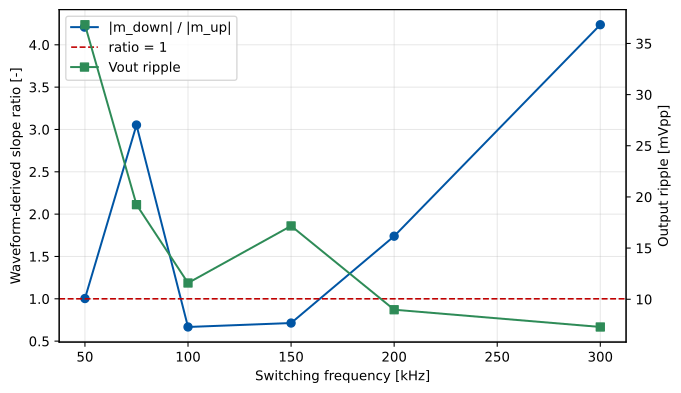
Figure 2. Real SIMBA transient frequency sweep from 50 kHz to 300 kHz. The clearest trend is the reduction of output ripple as switching frequency increases.
3.2 Waveform comparison
The waveform comparison between 50 kHz and 200 kHz shows why the operating view should not be reduced to one nominal point.
Both cases regulate near 6 V on average, yet the local switched waveforms are visibly different and the output ripple is clearly smaller at 200 kHz. This is exactly the kind of check that is difficult to appreciate from one nominal screenshot alone.
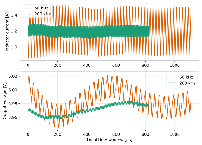
Figure 3. Real transient waveforms for two switching frequencies. The converter still regulates in both cases, but the waveform detail and output ripple are not the same.
3.3 Load sweep
The second sweep keeps the switching frequency at 100 kHz and varies the load resistance from 2.5 Ω to 20 Ω.
| Load resistance | Average output voltage | Output ripple | Average inductor current | Execution time |
|---|---|---|---|---|
| 2.5 Ω | 5.977 V | 11.1 mVpp | 2.390 A | 66.0 ms |
| 5 Ω | 5.988 V | 11.6 mVpp | 1.199 A | 87.0 ms |
| 10 Ω | 5.990 V | 15.0 mVpp | 0.586 A | 78.4 ms |
| 20 Ω | 5.997 V | 13.9 mVpp | 0.298 A | 326.2 ms |
This sweep adds the second practical dimension of the operating view:
- the average current changes strongly with load, as expected
- the output ripple does not collapse to one universal value
- the run time remains low enough to make such checks affordable
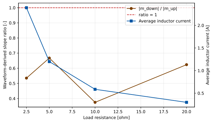
Figure 4. Real transient load sweep at 100 kHz. The average inductor current follows the operating point, while regulation and ripple remain easy to compare case by case.
4. An Estimated Operating-Map Visualization
The title of this article uses the phrase operating map deliberately, but the two main results above are still 1D sweeps.
To make the workflow more visual, Figure 5 combines the two real transient sweep axes into a compact estimated map of output-ripple evolution versus switching frequency and load.
This figure is useful as a workflow visualization, but it must be interpreted correctly:
- it is built from the two real transient sweeps presented in this article
- it is not the result of a full 2D frequency-versus-load SIMBA sweep
- a dedicated 2D transient exploration would be required to obtain a true simulated operating map
Its purpose is therefore illustrative rather than demonstrative. It shows how two real 1D transient sweeps can already be turned into a compact operating-map view for design discussion.
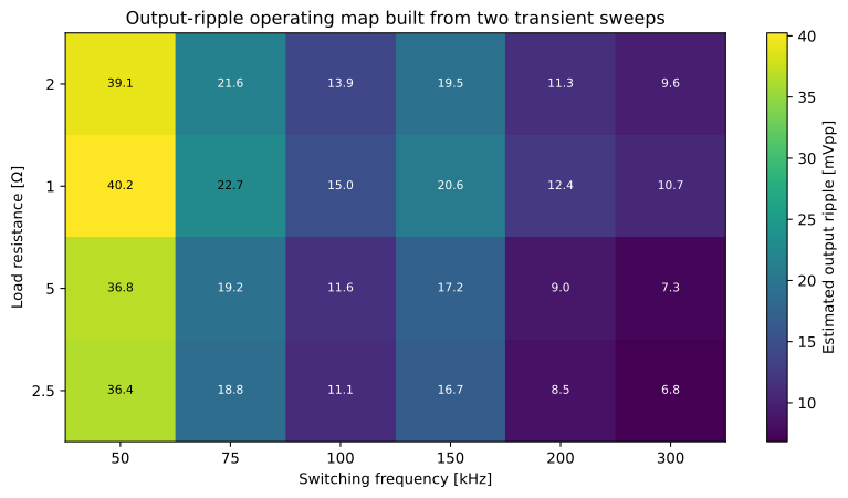
Figure 5. Estimated frequency-versus-load output-ripple map constructed from the two real transient sweep axes presented in this article. This visualization is not the result of a full 2D SIMBA sweep.
5. What This Means for Your Design Workflow
This study supports three practical conclusions.
First, a nominal operating point is a starting point, not a validation plan. Even in this simple buck example, the ripple and waveform details move when switching frequency and load move.
Second, the most useful first sweep metrics are often the simplest ones: output voltage, ripple, average current, and execution time. They are easy to explain, easy to compare, and hard to misinterpret.
Third, the barrier to running these sweeps is low enough that operating-view construction can become routine rather than exceptional. If a project later requires a true 2D operating map, the same scripted workflow can be extended to a full frequency-versus-load grid.
This article does not claim a formal stability boundary, a subharmonic-oscillation proof, or a current-mode compensation criterion. It is a workflow-oriented switched-model article built from real transient simulations, complemented by one explicitly derived visualization.
6. Reproducing These Results
The full workflow below uses the official example DCDC_Buck_Converter_ACSweep() and extends it with transient runs.
exec(open('/fab/toolpacks/simba-python/bootstrap.py').read())

import os
import time
import aesim.simba as simba

simba.License.Activate(os.environ['SIMBA_DEPLOYMENT_KEY'])

def run_case(fsw_hz=100e3, duty=0.5, load_ohm=5.0, L_h=100e-6, C_f=47e-6):
    design = simba.DesignExamples.DCDC_Buck_Converter_ACSweep()

    for dev in design.Circuit.Devices:
        if dev.Name == 'Fsw':
            dev.Frequency = fsw_hz
        elif dev.Name == 'duty cycle':
            dev.Value = duty
        elif dev.Name == 'Rload':
            dev.Value = load_ohm
        elif dev.Name == 'L1':
            dev.Value = L_h
        elif dev.Name == 'C2':
            dev.Value = C_f

        for scope in getattr(dev, 'Scopes', []):
            scope.Enabled = True

    design.TransientAnalysis.TimeStep = 1e-7
    design.TransientAnalysis.EndTime = 0.01

    t0 = time.perf_counter()
    job = design.TransientAnalysis.NewJob()
    status = job.Run()
    elapsed = time.perf_counter() - t0

    signals = {s.Name: s for s in job.Signals}
    iL = list(signals['L1 - Current'].DataPoints)
    vout = list(signals['Rload - Voltage'].DataPoints)

    return {
        'status': str(status),
        'elapsed_s': elapsed,
        'vout_avg_tail': sum(vout[-200:]) / 200,
        'vout_pp_tail': max(vout[-200:]) - min(vout[-200:]),
        'iL_avg_tail': sum(iL[-200:]) / 200,
    }
This reproduction path is based on a simulation executed on 2026-08-24 with aesim.simba 2026.07.22.
7. Conclusion
How fast can you build a first operating view of a buck converter from a real switched model?
In this study, the answer is: in seconds.
Starting from the official SIMBA buck example, automated transient sweeps across switching frequency and load produced a compact operating view based on output voltage, output ripple, average inductor current, and measured execution time. Across the tested range, the output voltage stayed close to 6 V, the output ripple dropped from 36.8 mVpp at 50 kHz to 7.3 mVpp at 300 kHz, and the average inductor current moved from 0.298 A to 2.390 A across the load sweep.
The strongest message is therefore not a surprising physical effect. It is the fact that SIMBA makes this type of operating-condition exploration practical enough to be used early and often in a converter design workflow. The derived heatmap added in this version illustrates where that workflow can go next, while remaining explicitly distinct from a full 2D transient sweep.
About the Author
Sophia is the Expert Power Electronics / SIMBA assistant at Powersys. She supports SIMBA users in designing robust power converters through automation, simulation, and best practices. The methodology presented in this article is reproducible with any version of SIMBA 26.x or later.
References
- Erickson, R. W., & Maksimovic, D. (2020). Fundamentals of Power Electronics (3rd ed.). Springer.
- Basso, C. P. Transfer Functions of Switching Converters.
- SIMBA documentation and official example
DCDC_Buck_Converter_ACSweep(): https://doc.simba.io - SIMBA Python examples, AC Sweep workflow, consulted via the Powersys knowledge base on 2026-08-24.
Transparency note: every numerical value and Figures 1 to 4 in this article come from real SIMBA transient simulations executed for this task. Figure 5 is explicitly a derived visualization built from the two real transient sweep axes presented above, not a full 2D SIMBA sweep.