Improve your workflow
Python is a powerful tool for scientific computing, control, and automation around simulation models.
Run SIMBA from Python scripts.
SIMBA Python Library is a Python package that lets users manage SIMBA from circuit creation to simulation and post-processing.
Python syntax is accessible, so the library can be used for simple scripts as well as for larger automation workflows.
Run simulations, inspect results, and document studies from a notebook-driven workflow.
The Python Library makes it easier to integrate SIMBA into analysis, scripting, and post-processing workflows.
Python is a powerful tool for scientific computing, control, and automation around simulation models.
SIMBA can be used from regular Python scripts or from notebooks for interactive studies and reports.
Simple Python loops make it easy to automate repeated simulations and compare results.
SIMBA can be combined with tools such as NumPy and Matplotlib for calculations, plots, and post-processing.
The examples below show how SIMBA can be controlled directly from Python.
# Load required module
from aesim.simba import Design
import matplotlib.pyplot as plt

# Create design
design = Design()
design.Name = "DC/DC - Buck Converter"
design.TransientAnalysis.TimeStep = 1e-6
design.TransientAnalysis.EndTime = 10e-3
circuit = design.Circuit

# Add devices
V1 = circuit.AddDevice("DC Voltage Source", 2, 6)
V1.Voltage = 50
SW1 = circuit.AddDevice("Controlled Switch", 8, 4)
PWM = circuit.AddDevice("Square Wave", 2, 0)
PWM.Frequency = 5000
PWM.DutyCycle = 0.5
PWM.Amplitude = 1
D1 = circuit.AddDevice("Diode", 16, 9)
D1.RotateLeft()
L1 = circuit.AddDevice("Inductor", 20, 5)
L1.Value = 1e-3
C1 = circuit.AddDevice("Capacitor", 28, 9)
C1.RotateRight()
C1.Value = 100e-6
R1 = circuit.AddDevice("Resistor", 34, 9)
R1.RotateRight()
R1.Value = 5
R1.Name = "R1"
for scope in R1.Scopes:
    scope.Enabled = True
g = circuit.AddDevice("Ground", 3, 14)

# Make connections
circuit.AddConnection(V1.P, SW1.P)
circuit.AddConnection(SW1.N, D1.Cathode)
circuit.AddConnection(D1.Cathode, L1.P)
circuit.AddConnection(L1.N, C1.P)
circuit.AddConnection(L1.N, R1.P)
circuit.AddConnection(PWM.Out, SW1.In)
circuit.AddConnection(V1.N, g.Pin)
circuit.AddConnection(D1.Anode, g.Pin)
circuit.AddConnection(C1.N, g.Pin)
circuit.AddConnection(R1.N, g.Pin)

# Run simulation
job = design.TransientAnalysis.NewJob()
status = job.Run()

# Get results
t = job.TimePoints
Vout = job.GetSignalByName("R1 - Instantaneous Voltage").DataPoints

# Plot curve
fig, ax = plt.subplots()
ax.set_title(design.Name)
ax.set_ylabel("Vout (V)")
ax.set_xlabel("time (s)")
ax.plot(t, Vout)Circuits can be created from scratch and modified with a few lines of Python: adding devices, placing them, connecting them, running the simulation, and retrieving results.
# Load required modules
import matplotlib.pyplot as plt
import numpy as np
from aesim.simba import DesignExamples

# Calculate Vout = f(duty cycle)
BuckBoostConverter = DesignExamples.BuckBoostConverter()
dutycycles = np.arange(0.00, 0.9, 0.9 / 100)
Vouts = []
for dutycycle in dutycycles:
    # Set duty cycle value
    PWM = BuckBoostConverter.Circuit.GetDeviceByName("C1")
    PWM.DutyCycle = dutycycle

    # Run calculation
    job = BuckBoostConverter.TransientAnalysis.NewJob()
    status = job.Run()

    # Retrieve results
    t = np.array(job.TimePoints)
    Vout = np.array(job.GetSignalByName("R1 - Instantaneous Voltage").DataPoints)

    # Average output voltage for t > 2 ms
    indices = np.where(t >= 0.002)
    Vout = np.take(Vout, indices)
    Vout = np.average(Vout)

    # Save results
    Vouts.append(Vout)

# Plot curve
fig, ax = plt.subplots()
ax.set_title(BuckBoostConverter.Name)
ax.set_ylabel("Vout (V)")
ax.set_xlabel("Duty Cycle")
ax.plot(dutycycles, Vouts)
Basic Python functions such as for loops are enough to automate parameter variations and
study their effect on simulation results.
SIMBA analyses can be launched directly from Python and integrated into larger workflows.
With the SIMBA Python Library, SIMBA simulations and pre- and post-processing can be integrated into one scriptable workflow.
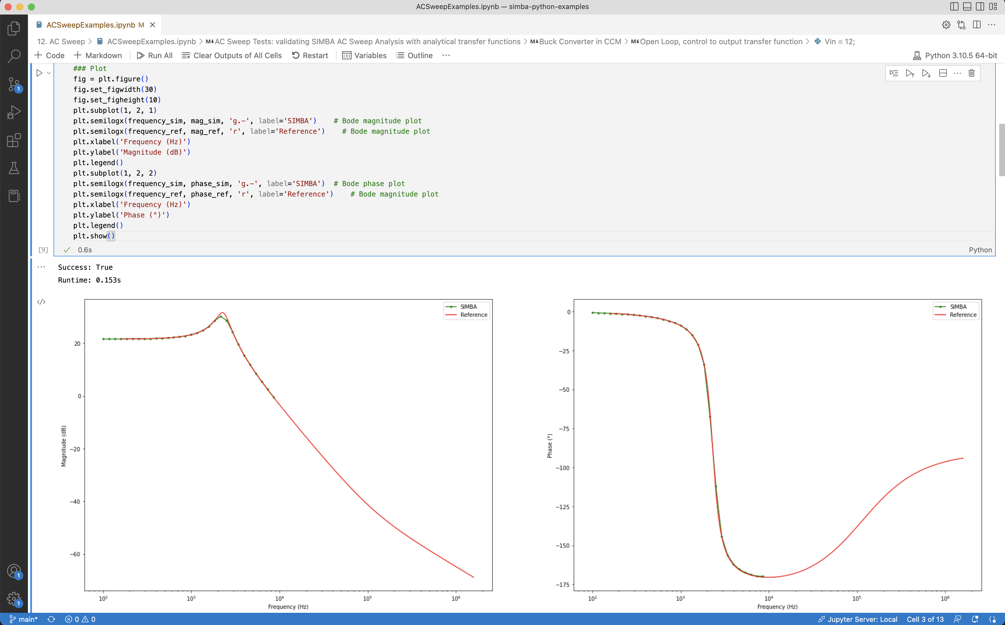
Different circuit analyses can be run from Python to obtain transient or steady-state waveforms, transfer functions, and impedances.
The Python Library is useful for automation, post-processing, and repeated simulation studies around SIMBA models.


© Copyright 2019-2026 – AESIM.tech | Privacy policy