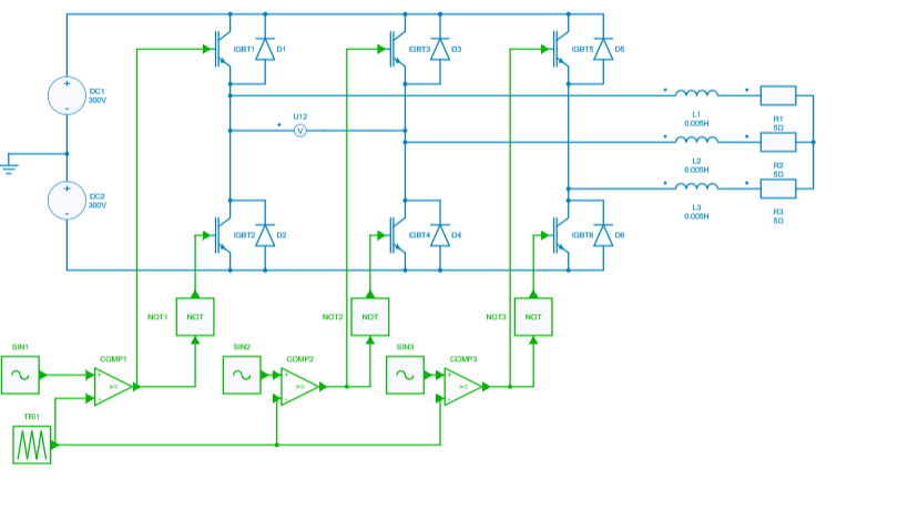
Three-phase-inverter: sweep of modulation depth $m$ depending on dc bus voltage $E$
import numpy as np
import xarray as xr
import pandas as pd
import os
import time as t

from scipy import signal

from aesim.simba import Design, ProjectRepository

from bokeh.plotting import figure
from bokeh.io import show, output_notebook
line_line_voltage = 300
fmod = 50
dc_bus_voltages = [800, 700, 600]
modulation_depths = 2 * line_line_voltage * np.sqrt(2) / dc_bus_voltages / np.sqrt(3)
project = ProjectRepository(os.getcwd() + R"\Test-emi.simba")
mycvs = project.GetDesignByName('three-phase-inverter')
vdc1 = mycvs.Circuit.GetDeviceByName('DC1')
vdc2 = mycvs.Circuit.GetDeviceByName('DC2')
pwms = [mycvs.Circuit.GetDeviceByName('SIN'+k) for k in ['1', '2', '3']]

res_time = []
res_u12 = []
res_iL = []

tic = t.process_time()
for dc_bus_voltage, modulation_depth in zip(dc_bus_voltages, modulation_depths):
    vdc1.Voltage = dc_bus_voltage / 2
    vdc2.Voltage = dc_bus_voltage / 2
    for pwm in pwms:
        pwm.Amplitude = modulation_depth
        pwm.Frequency = fmod
    job = mycvs.TransientAnalysis.NewJob()
    status = job.Run()
    res_time.append(job.TimePoints)
    res_u12.append(job.GetSignalByName('U12 - Instantaneous Voltage').DataPoints)
    res_iL.append(job.GetSignalByName('L1 - Instantaneous Current').DataPoints)
toc = t.process_time()
print('Elapsed time to simulate = ', toc - tic)
Elapsed time to simulate = 0.46875
# plot
TOOLTIPS = [
    ("index", "$index"),
    ("(t, val)", "($x, $y)"),
    ]

# figure 1
p1 = figure(plot_width = 800, plot_height = 300,
           title = 'Line-line voltage',
           x_axis_label = 'time (s)', y_axis_label = 'Voltage (V)',
           active_drag='box_zoom',
           tooltips = TOOLTIPS)
# figure 2
p2 = figure(plot_width = 800, plot_height = 300,
           title = 'Line current',
           x_axis_label = 'time (s)', y_axis_label = 'Current (A)',
           active_drag='box_zoom',
           tooltips = TOOLTIPS)

green_color = 50
for time, u12, iL in zip(res_time, res_u12, res_iL):
    p1.line(time, u12, color=(0, green_color, 0))
    p2.line(time, iL, color=(0, green_color, 0))
    green_color += 100

output_notebook()
show(p1)
show(p2)
# Prepare figure
TOOLTIPS = [
    ("index", "$index"),
    ("(freq, val)", "($x, $y)"),
    ]
p1 = figure(plot_width = 800, plot_height = 300,
           title = 'Frequency Spectrum',
           x_axis_label = 'frequency (kHz)', y_axis_label = 'Voltage (V)',
           active_drag='box_zoom',
           tooltips = TOOLTIPS)
green_color = 50
width = 0.02

# Prepare resampling
N = 10000
time_resamp = np.linspace(0, 2 / fmod, 2 * N, endpoint=False)

for time, u12 in zip(res_time, res_u12):
    # resampling for fft
    u12_resamp = np.interp(time_resamp, time, u12)
    fstep = 50    # consider only N points of the 2N point resampled vector
    time_resamp_window = time_resamp[N:]
    u12_resamp_window = u12_resamp[N:]

    # do fft
    freq = np.fft.fftfreq(N) * fstep * N
    positivefreq = freq[freq >= 0]
    freqval = np.abs(np.fft.fft(u12_resamp_window)) / N
    freqval[1:] = freqval[1:] * 2
    freqval = freqval[freq >= 0]

    # Get only 300 harmonics
    max_index = 300
    positivefreq = positivefreq[:300]
    freqval = freqval[:300]
    p1.vbar(x=(positivefreq/1e3), width=width, bottom=0, top=freqval, color=(0, green_color, 0))
    green_color += 100
    width *= 0.5

show(p1)